Abstract: Divergence is an understudied subject loosely defined as an unpredictable random error. The classification of divergences as small or large is also at the heart of efficient or inefficient market theory debate. This paper explains how divergence is cyclical and can be quantified and used as a predictive model.
Keywords: divergence, cyclicality, relative performance, rate of change, assets, rank, distribution
Smith, Pareto and the divergence debate.
Life is all about making sense of information. This information could be personal, economic, or societal kind. When we comprehend information, we make a decision, which we assume to be correct. So, at a certain level, we try to understand performance and how to perform as individuals to make performing choices. Performance assumes a kind of order. We try to create order in decision making from disorder in the external world. This disorder could also be called divergence. Divergence is a phenomenon seen in nature and markets. It is something that needs explaining and can be unexplainable at times. It is linked with change or rate of change1. Divergence is also assumed to be random2. Divergence happens as prices move away from a theoretical value calculated statistically or fundamentally3. Divergence is not considered normal. Divergence is also known as non confirmation in technical analysis4 (the study of market patterns). Divergence also creates news, as something that is not normal is strange and worth talking about. For example when company beat analyst expectations (disappoint) and there are large changes in price action. Divergence can be seen in information and data also.
Adam smith5 (1723-1790) talked about the invisible hand, what we don’t know something unpredictable, a kind of divergence. Vilfredo Pareto6 (1848-1923) talked about non homogeneous wealth allocation. 80% of the wealth is with 20% of people. This unequal allocation was a divergence. Charles Dow7 (1851-1902) talked about a basic tenet of markets in his now famous Dow Theory. If Dow industrials8 and Dow Transports9 were not moving together, it was a non confirmation10, a case of divergence. Dow Industrials made higher high in January 2000, while Dow transports did not. Divergence case was indicated by Charles Dow as a reason for divergence. Markets changed trend after the respective divergence. Ralph N Elliott11 (1871-1948) talked about truncation12, double extension13, throw over as rare (divergent, non normal) rare formations in classic Elliott wave theory. Edward Norton Lorenz14 (1917 – 2008) talked about Chaos and how small changes in early conditions lead to totally new behavior (unpredictable divergent behavior), leads to the butterfly effect.
We can see cases of divergences in current times. John Murphy15 talked about linkages between markets and assets. Gold and dollar generally move opposite. When Gold strengthens, dollar weakens and vice versa. There are times when gold and dollar don’t follow this relationship Murphy calls it an Intermarket failure. Sam Stovall16 talked about sector performance divergences. Sector price performances vary as the economic cycle changes. There is a stage in the economic cycle when Utility sectors outperform financials and there is a stage in the economic cycles when utility sectors underperform financial sector. Putting simply sector differ or diverge in performance from each other in different times.
Robert Shiller17 talked about divergence between market data and fundamental value as earnings don’t have a commensurate effect on price performance. Shiller fluctuations are divergence cases. Mandelbrot18 talks about extremities, large divergences which cannot be explained by the normal distribution Gaussian curve. Nassim Taleb19 says black swan is random, rare, unpredictable, an extreme divergence.. Robert Arnott20 talks about how growth diverges from value and creates cyclical opportunities. Robert Prechter21 has done extensive work on social mood divergences; rising hem of skirts, films we watch, sugar we consume, social mood diverges from one extreme to other.
The inefficient22 market school of thought is based on large divergences while the efficient market school of thought is based on small divergences. Coming to look at it the debate between market efficiency and inefficiency, revolved around divergence. If it is small, it is normal distribution, if it’s large, it’s inefficient and exponential distribution.
Large divergence is a reality between high, low, negative correlated assets. For example there was a 60% net change in price performance between gold and palladium from July 2009 till January 2010 and 55% between Brent23 and Exxon24 from July to October 2008. Even 100% divergences between sector peers are not too rare. They happen regularly.
How can we define large divergence? Is small divergence any less important than the case of large divergence? Sam Stovall sector rotation outperformance and underperformance can be seen as divergence of 12% net change in price performance between Dow Industrials and Dow Financials from October to November 2009. Stovall did not discuss small consistent repeating semiannual divergences of 5% between Dow Industrials and S&P 500. Small divergences are as important as large 100% repeating divergences between two sectors. Behavioral finance25 talks about divergences as anomalies that are tough to capture. Is it because divergences are tough to isolate, measure, explain, quantify?
Robert Shiller explains why markets are inefficient using various time series of present value of dividends and plotting them against stock prices illustrating more than normal fluctuations. His proof that markets are inefficient is based on the fact that large divergences can’t be explained. Divergences are everywhere, in capital markets, economics, sciences and we still consider them somehow non forecastable, extremities, errors, non normal behavior, non ordered, and chaotic.
To understand divergence one can go back in the history of how data interpretation evolved. Mandelbrot said nature was full of extreme divergences and the Gaussian bell curve had more fat tails that it could explain. The divergences from mean were large. Though Mandelbrot was correct as divergences in nature were large and divergences on occasions don’t revert to mean, but the question to be asked is why did Gauss not see the large divergences from mean? There could be many reasons. Could it be because Gauss was handling Astronomical data, which was more ordered than other data found in nature? Or maybe because data interpretation was a nascent science and hence the first obvious visual pattern Gauss could see was the mean line.
As time passed and data interpretation came off age, the size, quality and quantity of data enhanced. There was more data to fit, a lot of it. The attention moved from data to divergence in data. Larger the divergences became visible, fatter the tails26 became. Whatever was Gaussian suddenly started to look exponential.
We, as humans, are somehow not designed to understand extremes, but mean and average. The society understands average salary, average GDP and so on. Average has safety, comfort, which extremes lack. Technical analysts are familiar with moving average but a majority of us can’t visualize the average27, which is always changing, mixing, transforming. A lot of other parameters extend from the idea of mean. What would happen to correlation if the mean was dynamic? Small divergence around the mean was considered efficient and large divergence made everything inefficient.
The first question one may ask about historical and contemporary divergence cases is if these divergences are cyclical. John Murphy states that Intermarket linkages are cyclical, as money moves from soft to hard assets and from commodities to bonds. Sam Stovall’s economic sectors cyclically move in and out of performance. There is repetitiveness in sector rotation, cyclicality in divergence. Robert Shiller’s case of bubble formations is cyclical. Mandelbrot’s repeating extremities and Nassim Taleb’s recurring random events are periodic. Repeating extremities are the reason fractal geometry and butterfly effect exists.
Taleb’s Black swan is a subject of study because there is not only one black swan. The black swans come again and again, periodically. Robert Arnott’s investing out of growth into value and vice versa is cyclical. Robert Prechter’s social mood diverges cyclically positive mood to negative mood and back. Behavioral Finance talks about investor’s errors and repeating Long reversals. The subject of behavioral finance would not be valuable if long reversals didn’t repeat.
Top performers underperform and top underperformers also perform. Dow Industrials underperforms S&P 500 and vice versa. Similar cyclicality can be seen between gold and copper. Gold underperforms and outperforms copper cyclically, the pairs diverging 8% to 10% cyclically in a quarter28. Small and large divergences are cyclical. Divergence cyclicality introduces an order in divergence. Because the focus was around mean, everything around mean was considered noisy and extreme. The idea of divergence cyclicality is a study of extremities, the study of cyclicality of error, it also proves that mean could be more dynamic than believed.
Clifford Pickover29 in his book “The math book” tells us that “Simple computer programs, which attempt to find regularity in sequences, may not “See” the regularity in Champernowne’s number30. This deficit reinforces the notion that statisticians must be very cautious when declaring a sequence to be random or patternless.
On one side Mandelbrot’s idea of extremity robs us of the beauty of the bell shaped curve, and on the other side it’s the same bell curve, which is used to disprove patterns in nature.” The paradox is very sad. We are busy debating about randomness and order never even once thinking of the error that creates it all. Divergence cyclicality can reconcile the efficient and inefficient school of thought. It can explain that both Gauss and Mandelbrot are talking about the same mean. But it’s Mandelbrot who takes the argument to the next level by assuming larger divergence around mean as more important than the smaller divergence around the mean. Both of them speak about mean reversion31, one saying it works, while the other refutes it.
Divergence cyclicality on the other hand is more focused on defining a pair, a group, than defining an average. Divergence cyclicality can be the new predictive model that takes data interpretation to the next level, by introducing time cyclicality into data and suggesting that the basic pattern of order (small divergence) or randomness (large divergence) is cyclical.
Quantifying Divergence.
Human beings are always ranking choices. Though this intuition seems like a system, rankings between a group of people can show a lot of variability as the process of ranking is individual, non standardized and emotional. Humans also try to understand by grouping assets or parameters together. They try to look for similar features, characteristics and this is why economies, regions, political affiliations are grouped. BRICS, MAVINS32 and PIGS is an example of grouping associated with similar ranking economies. The global competitiveness report is a ranking process on global economies on a host of parameters (World Economic Forum, “The Global Competitiveness Report 2009-2010”).
Though this intuitive ranking reflects in the investment process, majority prefers absolute over relative performance. There is less news on relative performance but more on absolute performance. “Gold made a new high today” can be an investment news but “gold outperformed silver by 10% in the last quarter” is rarely published. Investment portfolios rarely get benchmarked to other assets like dollar or gold to understand year to date relative performance against key global benchmarks.
Investors use a similar ranking and grouping process to diversify, but maybe because the comfort and confidence is low regarding this ranking and grouping system that the majority investors diversify less. Behavioral finance highlights that investors diversify less (Modern Portfolio Theory and Investment Analysis by E. Elton, M. Gruber and others”). Diversification is also suggested as an action point to reduce risk but owing to limited diversification and inability to benchmark portfolio performance investors are unable to comprehend a macro portfolio of global assets on a relative basis are more prone to geographical biases.
The majority of investors fail to understand that the assets traded today are also paired against a currency. Dow Industrials (.DJI) is paired against dollar and Sensex is paired against Indian Rupee, Nikkei is paired against Yen. Even EURUSD is a pair made from two currencies. Yield curves are studied to understand interest rate trend. A yield curve is a spread between long term and short term interest rates.
Pair ideas are everywhere whether we speak about Risk vs. Return, Demand for cash vs. Demand for assets, Risk aversion vs. loss aversion, Pessimism vs. Optimism, Perceived risk vs. actual risk, Relative vs. Market Value, PE (Price Earning Multiple) vs. Market Value, Liquidity vs. Solvency ratios, Supply vs. Demand.
Pair trading is an active strategy globally because it offers an opportunity to capture divergence. We studied divergence in various pairs and one could see increasing and decreasing divergence patterns. We made a case of Boeing and Oil (Brent) and exhibited a case of divergence cyclicality. Visually one could identify lows and highs in divergence and the no divergence stage.

Figure 1: Boeing and Oil (Brent) divergence cyclicality
Source: Authors work. Data provided by Thomson Reuters
Divergence analysis, a study of cyclicality as relative performance or spread analysis has no units, it is a statistical ratio. Divergence analysis connects ranking, pairs and relative performance. Relative performance is the price performance of one asset netted against performance of another asset. The two compared assets can be a stock against its Index, a sector index against another sector Index, a portfolio against the composite index etc. Relative performance can also be understood as alpha. A negative relative performance is underperformance while a positive relative performance is outperformance. It can be constructed with the following steps.
The data for an Index and its constituents are collected in the following format. The asset and its benchmark are compiled together. In this case the closing price data of Dow Jones Industrial Average (DJIA) is plotted along with the closing price of its components like Alcoa. This is illustrated in table 1.
Table 1. Closing prices for Dow, Alcoa, Disney, Dow, Walmart

Table2. Ratio between the price and the benchmark

Source: Authors work. Data provided by Thomson Reuters
In table 3, a 60 period averaging is done to look at quarterly tendency in daily change in relative performance values. Alcoa table 3 value for 4 Apr 08 = Alcoa (9Jan table2 value+10 Jan table2 value+ …+3Apr table 2 Value)/60
Table 3. 60 days period moving average on data

Source: Authors work. Data provided by Thomson Reuters
We plotted a rate of change (ROC) on this relative performance. ROC is an indicator that shows the difference between today’s closing price and the close price N days ago. It is also referred to as momentum and can be understood as the absolute difference: Rate of change can also be represented as a fraction. ROC plotted on relative performance was an improvement on illustrating divergence cyclicality. We employed this process in our paper. This was an attempt to quantify divergence. To qualify one signal from the other we had to find a way to focus on extreme divergences. The larger the divergence we could isolate, the better we could quantify it. This was when we decided to look at divergence in a group of assets because a group divergence is higher than a pair divergence. The group focus helped us intensify extremes. To create groups we used relative performance and we ranked them.
Ranking the assets.
We integrated a global portfolio with the following 54 assets. Forex (EUR USD, AUD USD, GBP USD, CAD USD, JPY USD, CHF USD, Yuan Rnmbi, Indian rupee, NZD USD), Energy (Crude, Natural Gas, Gasoline, Heating Oil, Petroleum, Carbon Emissions, Brent, WTM, Energy Index), Metals (Precious Metals, Tin, Zinc, Nickel, Copper, Platinum, Silver, Industrial Metals Index, Gold), Agro (Coffee, Corn, Grains, Livestock, Sugar, Wheat, Soybeans, Cotton), Thematic and Global Equity (Coal Mining Fund, Shipping Fund, Dow Industrials, Sense, Agricultural Equity, Water, Nuclear, Russell 2000, Russell 1000 USD), Bonds (US 30, US 5Y, US 10Y, US 2Y, INR Bond Index, China Bond Index, Australian Bond Fund, Global Bond Index, Sweden Bond Index) and benchmarked the portfolio to dollar.
Figure 2. Global portfolio of 54 assets

Source: Authors work. Data provided by Thomson Reuters
We numerically ranked33 the portfolio according to assets, sectors and on aggregate bases. Now we could not only see the top performers and worst performers but also how rankings were dynamic. The worst was becoming the best and vice versa. We could now qualify one divergence low from the other. The best ranked asset paired up with the worst was a divergence extreme that could indicate performance cyclicality. And since divergence did not differentiate between assets, we could even talk about performance cyclicality between zinc and coffee, suggesting that zinc should outperform coffee as coffee was the top ranked and Zinc the worst and divergence (performance was cyclical). This dynamic performance when plotted as a time series took the form of an oscillator. The dollar oscillator illustrated below suggested dollar outperformance against various forex pairs and vice versa as it moved from one extreme to another.
Figure 3. Dynamic performance (as oscillator for dollar)

Source: Authors work. Data provided by Thomson Reuters
Instead of histograms for one date we plotted the historical data for just one asset, Bank of America. A smoothing using two moving averages of 20 and 30 days elucidates the cyclical nature. The oscillator shows how the stock moves up in performance against DJIA and rest of the 29 components (the benchmark) and vice versa. When the oscillator hits the bottom the stock has hit underperformance low against DJIA and hence should reverse and start outperforming. On the other hand if the oscillator touches a high or tops, the stock has reached the top of its outperformance against DJIA. The stock should now reverse its performance and start underperforming DJIA. The image below suggests a start of outperformance for Bank of America against DJIA.
Figure 4. Bank of America asset’s relative performance oscillator

Source: Authors work. Data provided by Thomson Reuters
The numeric ranking and relative performance cyclicality opened up many other advantages. We looked at Hedge Efficiency when we paired the index against it future (Derivative). Using the ranking and performance cyclicality approach we could identify that the real time to hedge was when futures were underperforming the spot prices or in other words the divergence reached an extreme between the two assets. We tested the Nifty (Indian Index) against its Future and isolated more than a risk free return consistently.
Fig.5. Hedge efficiency
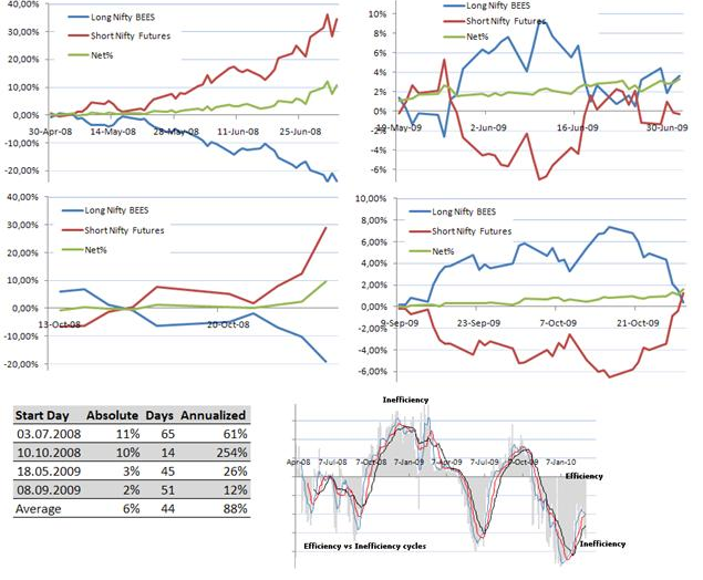
Source: Authors work. Data provided by Thomson Reuters
Cases. Fig. 6a. 6b. 6c. 6d- Asset Energy – Exxon (benchmarked with Brent)

Source: Authors work. Data provided by Thomson Reuters
Cases. Fig. 6a. 6b. 6c. 6d- Asset Energy – Exxon (benchmarked with Brent)

The Relative performance oscillator (Fig 6e.) for Exxon indicates outperformance against Brent if the oscillator turns up and vice versa. We have tabulated four turn points. From 03 July 08 to 17 (arrow 1 to 2) Sep 2008 Exxon bet outperformed Brent by 52%. In this period Brent fell 63% while Exxon dropped just 11%. Similarly when the oscillator turned down Exxon underperformed Brent by 24%. The two cases are illustrated above in Fig.6a, Fig.6b, Fig.6c and Fig.6d. The table below carries individual performance and net performance between the two assets.

Source: Authors work. Data provided by Thomson Reuters
Conclusion.
The reason for the divergence debate is because divergence is ubiquitous. It is how nature and markets function. Divergence cyclicality drives this growth and decay process. Divergence cyclicality is also the reason markets keep moving from efficiency to inefficiency. History of research did not make an effort to understand divergence as it was thought to be noise, error which cannot be used as a predictive model. This paper proved that divergence can be understood by grouping assets and ranking them. This way extreme and large divergences not only become more comprehendible but also quantifiable. This quantification can be used to pin point performers and underperformers around the world whether it’s a social trend, economic regional cycle or traded assets. Divergence cyclicality is a predictive model that can change how we understand nature and markets.
Download the paper from SSRN.